Westmere-EP to Sandy Bridge-EP: The Scientist Potential Upgrade
by Ian Cutress on March 4, 2013 9:30 AM EST- Posted in
- CPUs
- Xeon
- Westmere-EP
- Sandy Bridge-EP
Grid Solvers
For any theoretical evaluation of physical events, we mathematically track a volume and monitor the evolution of the properties within that volume (speed, temperature, concentration). How a property changes over time is defined by the equations of the system, often describing the rate of change of energy transfer, motion, or another property over time.
The volume itself is divided into smaller sections or ‘nodes’, which contain the values of the properties of the system at that point. The volume can be split a variety of different ways – regularly by squares (finite difference), irregularly by squares (finite difference with variable distance modifiers), irregularly by triangles (finite element) to name three, although many different methods exist. More often than not the system has a point of action where stuff is happening (heat transfer at a surface or a surface bound reaction), meaning that some areas of the system are more important than others and the grid solver should focus on those areas (benefits against regular finite difference). This usually comes at the expense of increased computational difficulty and irregular memory accesses, but affords faster simulation time having to calculate 1000 variable distance points rather than 1 million (as an example of a 106 simulation volume). Another point to note is that if the system is symmetrical about an axis (or the center), the simulation and grid chosen is often reduced by a dimension to improve simulation throughput (as O(n) < O(n2) < O(n3)).
Boundary conditions can also affect the simulation – because the volume being simulated is finite with edges, the action at those edges has to be determined. The volume may be one unit of a whole, making the boundary a repeating boundary (entering one side comes out the other), a reflecting boundary (rate of change at the boundary is zero), a sink (boundary is constantly 0), an input (boundary is constantly 1) or a reactive zone (rate of change is defined by kinetics or another property) – again, there are many more boundary conditions depending on the simulation at hand. However as the boundary conditions have to be treated differently, this can cause extended memory reads, additional calculations at various points, or fewer calculations by virtue of constant values.
A final point to make is dealing with simulations involving time. For the scenarios I simulated in research, time could either be dealt with as a pushing structure (every node in the next time step is based on the surrounding nodes ‘pushing‘ the values of the previous time step) or pulling structure (each calculation of the next time step requires pulling a matrix of values from the previous time step), also known as explicit and implicit respectively. By their nature, explicit simulations are embarrassingly parallel but have restricted conditions based on time step and node size – implicit simulations are only slightly parallel, require larger memory jumps but have several fewer restrictions that allow more to be simulated in less time. Deciding between these two methods is often one of the first decisions when it comes to the sorts of simulation I will be testing.
All of the simulations used in this article were described in our previous GA-7PESH1 review in terms of both mathematics and code. For the sake of brevity, please refer back to that article for more information.
Explicit Finite Difference
For any grid of regular nodes, the simplest way to calculate the next time step is to use the values of those around it. This makes for easy mathematics and parallel simulation, as each node calculated is only dependent on the previous time step, not the nodes around it on the current calculated time step. By choosing a regular grid, we reduce the levels of memory access required for irregular grids. We test both 2D and 3D explicit finite difference simulations with 2n nodes in each dimension, using OpenMP as the threading operator in single precision. The grid is isotropic and the boundary conditions are sinks.
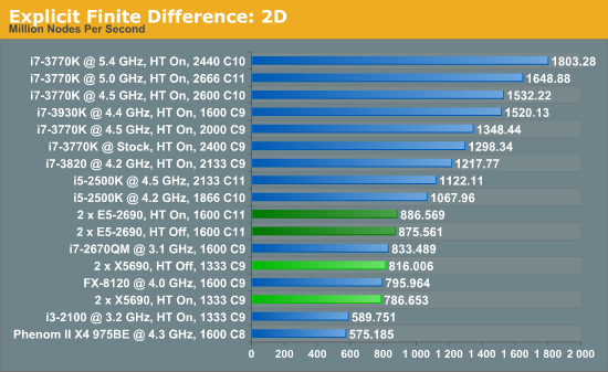
The 6-core X5690s in this situation definitely perform lower than the 8-core E5-2690s, although with the X5690s it pays to have HyperThreading turned off or face 3.5% less performance. Compared to the E5-2690s, the X5690s only perform 8% down for that 25% price difference.
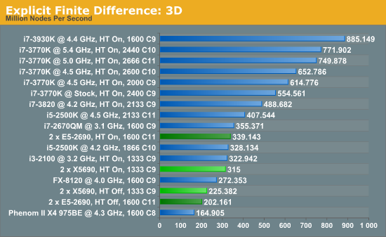
In three dimensions, the E5-2690s still have the advantage, at 7.7% with HT enabled. With HT disabled, the dual X5690 system performs 11.4% better than the Sandy Bridge-E counterparts. The nature of the 3D simulation tends towards a single CPU system performing much better, however.
Implicit Finite Difference (with the Alternating Direction Implicit method)
The implicit method takes a different approach to the explicit method – instead of considering one unknown in the new time step to be calculated from known elements in the previous time step, we consider that an old point can influence several new points by way of simultaneous equations. This adds to the complexity of the simulation – the grid of nodes is solved as a series of rows and columns rather than points, reducing the parallel nature of the simulation by a dimension and drastically increasing the memory requirements of each thread. The upside, as noted above, is the less stringent stability rules related to time steps and grid spacing. For this we simulate a 2D grid of 2n nodes in each dimension, using OpenMP in single precision. Again our grid is isotropic with the boundaries acting as sinks.
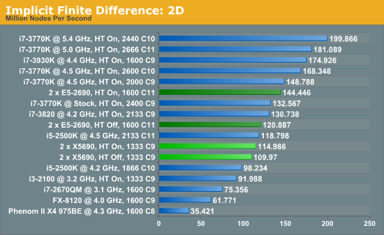
The IPC and increased memory bandwidth of the E5-2690 system comes through here, with the X5690s being 20% slower. The dual CPU nature of the system is still at odds with the coding, as a single i7-3930K at stock should perform similarly.


44 Comments
View All Comments
SatishJ - Monday, March 4, 2013 - link
It would be only fair to compare X5690 with E5-2667. I suspect in this case the performance difference would not be earth-shattering. No doubt E5-2690 excels but then it has advantage of more cores / threads.wiyosaya - Monday, March 4, 2013 - link
There is a possible path forward for those dealing with "old" FORTRAN code. CUDA FORTRAN - http://www.pgroup.com/resources/cudafortran.htmI would expect that there would be some conversion issues, however, I would also expect that they would be lesser than converting to C++ or some other CUDA/openCL compliant language.
As much as some of us might like it to be, FORTRAN is not dead, yet!
mayankleoboy1 - Monday, March 4, 2013 - link
1. Why not use 7Zip for the compression benchmark ? Most HPC people would like to use a FREE, Highly threaded software for their work.2.Using 3770K @ 5.4 Ghz as a comparison point is foolish. Any Ivy bride processor above ~4.6 on air is unrealistic. And for HPC, no body will use a overclocked system.
Senti - Monday, March 4, 2013 - link
WinRar is interesting because it's very sensitive to memory subsystem (7zip is less so), but 3.93 is absolutely useless as it utilizes about half of my cpu time and the end result it turns into powersaving impact benchmark before anything else. AT promised to upgrade sometime this year, but before it we'll continue to have one less useful benchmark.Not overclocking your cpu when you have good cooling is plain waste of resources. Of course I mean not extreme overclocks, but permanent maximum "turbo" frequency should be your minimum goal.
SetiroN - Monday, March 4, 2013 - link
Sorry but...-So what?
Being "sensitive to memory" doesn't make a worse benchmark better, or free;
-So what?
Nobody will ever have good enough cooling to be able to compute daily at 5.4, which is FAR above max turbo anyway. Overclocked results are welcome, provided that I don't need an additional $500 phase change cooler and $100+ in monthly bills.
tynopik - Monday, March 4, 2013 - link
> Being "sensitive to memory" doesn't make a worse benchmark better, or free;It makes it better if your software is also sensitive to memory speed
different benchmarks that measure different aspects of performance are a GOOD thing
Death666Angel - Monday, March 4, 2013 - link
The OC CPU I see as a data point for his statement that some workloads don't require multi socket CPU systems but rather a single high IPC CPU. It may or may not be unrealistic for the target demographic, but it does add a data point for or against such a thing.IanCutress - Tuesday, March 5, 2013 - link
1. WinZip 3.93 has been part of my benchmark suite for the past 18 months (so lots of comparison numbers can be scrutinized), and is the one I personally use :) We should be updating to 4.2 for Haswell, though going back and testing the last few years of chipsets and various processors takes some time.2. My inhouse retail CPU does 4.9 GHz on air, easy :) But most of the OC numbers are courtesy of several HWBot overclockers at Overclock.net who volunteered to help as part of the testing. For them the bigger score the better, hence the overclocks on something other than ambient.
Ian
mayankleoboy1 - Monday, March 4, 2013 - link
How many real world workloads are using hand-coded AVX software ?How many use compiler optimized AVX software ?
What is the perf difference between them?
Not directly related to this article, but how many softwares have the AMD Bulldozer/piledriver optimised FMA and BMI extensions ?
Kevin G - Monday, March 4, 2013 - link
What is going on with the Explicit Finite Difference tests? The thing that stood out to me are the two results for the i7 3770K at 4.5 Ghz with memory speed being the differentiating factor. Going from 2000 Mhz to 2600 Mhz effective speed on the memory increased performance by ~13% in the 2D tests and ~6% in the 3D tests. Another thing worth pointing out is that the divider in Ivy Bridge has higher throughput than Sandy Bridge. This would account for some of the exceedingly high performance of the desktop Ivy Bridge systems if the algorithms make heavy use of division. The dual socket systems likely need some tuning with regards to their memory systems. The results of the dual socket systems are embarrassing in comparison to their 'lesser' single socket brethen.The implicit 2D test is similarly odd. The odd ball result is the Core i7 3820@4.2 Ghz against the Ivy bridge based Core i7 3770k@stock (3.5 Ghz). Despite the higher clock speed and extra memory channel, the consumer Sandy Bridge-E system loses! This is with the same number of cores and threads running. Just how much division are these algorithms using? That is the only thing that I can fathom to explain these differences. Multi-socket configurations are similarly nerfed with the implicit 2D test as they are with the explicit 2D test.
Did the Browian Motion simulations take advantage of Ivy Bridge's hardware random number generator? Looking at the results, signs are pointing toward 'no'.
I'm a bit nitpicky about the usage of the word 'element' describing the n-Body simulation with regards to gravity. The usage of element and particle are not technically incorrect but lead the reader to think that these simulations are done with data regarding the microscopic scales, not stellar.
The Xilisoft Video Converter test results seem to be erroneous. More than doubling the speed by enabling Hyperthreading? How is that even possible? Best case for Hypthereading is that half of the CPU execution resources are free so that another thread can utilize them and get double the throughput. HT rarely gets near twice as fast but these results imply five times faster which is outside the realm of possibility with everything else being equal. Scaling between the Core i7-3960k and the dual E5-2690 HT Off result looks off given how the results between other platforms look too.